Terminology explained: P10, P50 and P90

When working with Monte Carlo simulations, some parameters that show up quite a lot are the P10, P50 and P90.

SHARE:

What are these parameters? Why are they so important?

The large amount of data produced by statistical methods sometimes make it difficult to effectively use its results in the decision-making process. As we mentioned in our post about the Monte Carlo method, this methodology is based on “simulating” potential scenarios. An example of its use in the oil and gas industry is the estimation of potential lifecycle (i.e. a feasible representation of the life of the asset) to predict asset performance. Sometimes, when running models with a large variation, analysts will engage simulations that go beyond 1000 lifecycles. This number multiplied by the specified period required to simulate the asset performance (i.e. platform useful life = 10-20 years) means that we are effectively tracking tens of thousands of years of simulation.

The P10, P50 and P90 are useful parameters to understand how the numbers are distributed in a sample. Let’s try to explain that using an example.

Consider the following sample (list of observations). They could represent anything – oranges, bananas, production efficiency etc.:

1. 95
2. 95
3. 96
4. 95
5. 97
6. 93
7. 94
8. 95
9. 96
10. 94

There are several options to display this data. You could decide to group the observations within a certain range and create a frequency table (i.e. how frequently an observation appears in the sample). This is calculated by counting the observations with a specific value and dividing by the total number of observations (e.g. 93 appears one time in a sample which has ten observations so its frequency is 10%):

Data	Number	Frequency
93	1	10%
94	2	20%
95	4	40%
96	2	20%
97	1	10%

The frequency can also be used to create the famous “bell” curve.

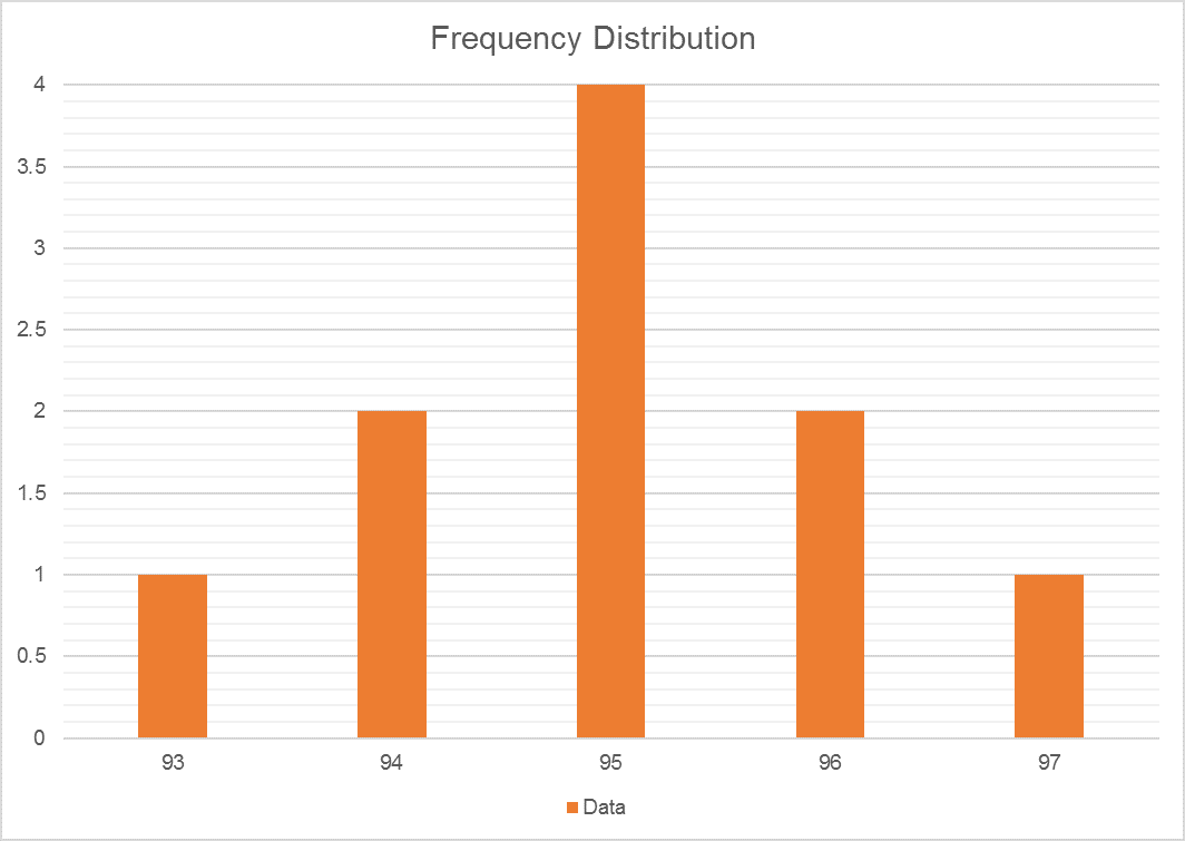
Normal distribution i.e. Bell curve

With this distribution, there is no need to have access to all the data points in the sample to start the inference work. We can tell, by looking at the graph, that most observations are around 95.

What is cumulative frequency and probability of exceedance and non-exceedance?

Another option to display this distribution is using a “Cumulative Frequency” graph. This table is calculated by adding each frequency from a frequency distribution table to the sum of its predecessors.

One will notice that you can start from either the lower observation values to higher observation values or the opposite. So, we must introduce two new concepts:

• Probability of exceedance: If you start from the left (i.e. lower observation values) of the bell curve to the right (i.e. higher observation values), you are building-up a probability of exceedance curve.
• Probability non-exceedance: If you start from the right (i.e. higher observation values) of the bell curve to the left (i.e. lower observation values), you are building-up a probability of non-exceedance curve.

So, considering our sample, if we are preparing a probability of exceedance graph, we know that 97 appears 10% of the time and 96 appears 20% of the time, so for a Cumulative Frequency distribution, we will have 96 associated to 30%. It means that 30% of the observations will exceed the value of 96.

Data	Number	Frequency	Probability of exeedence
93	1	10%	100%
94	2	20%	90%
95	4	40%	70%
96	2	20%	30%
97	1	10%	10%

 

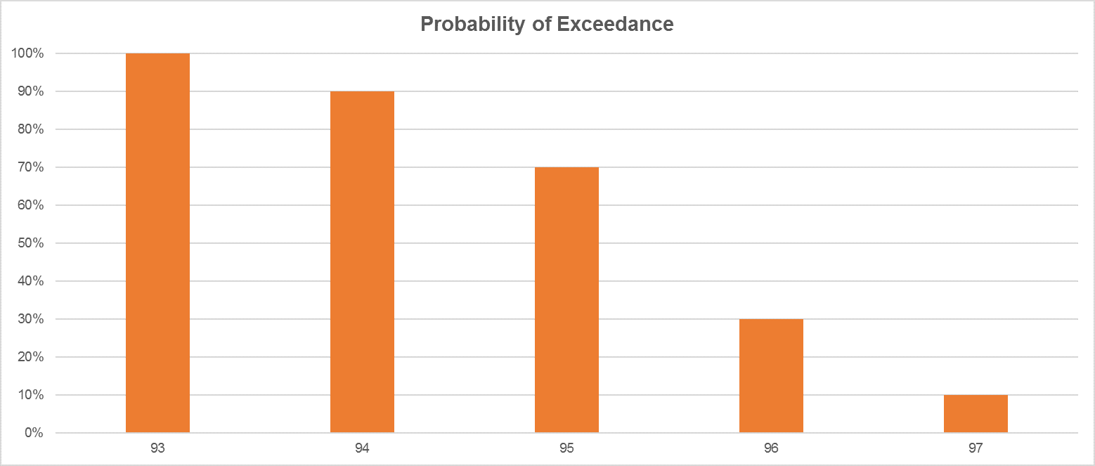
Probability of exceedance

Again, this graph adds up the frequency of occurrence as the value of the observation decreases i.e. 30% of our observations will be equal exceed the value of 96. This is what is called the probability of exceedance.

As mentioned before, another option is taking the opposite view – adding frequency of observations that will not exceed a certain value of observation.

So, considering our sample, if we are preparing a probability of non-exceedance graph, we know that 93 appears 10% of the time and 94 appears 20% of the time, so for a Cumulative Frequency distribution, we will have 94 associated to 30%. It means that 30% of the observations will be equal or not exceed the value of 94.

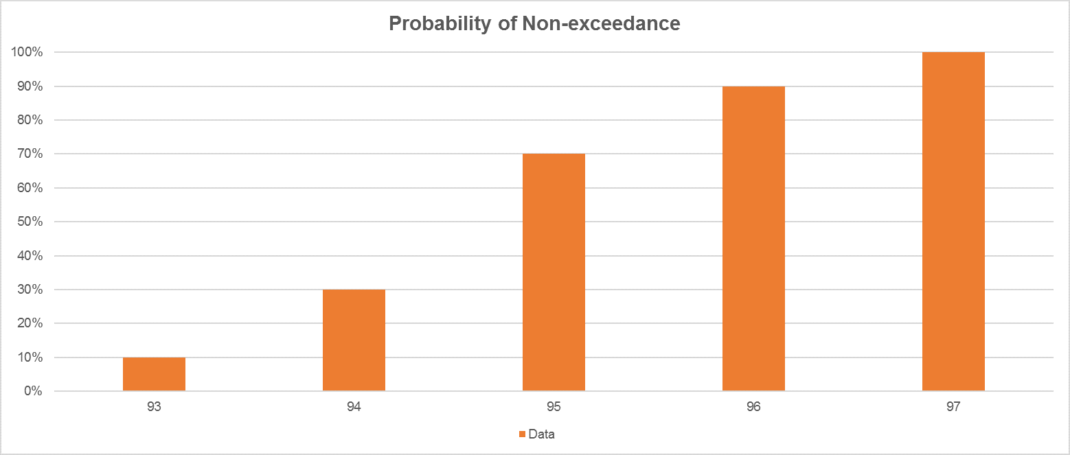
Probability of non-exceedance

Data	Number	Frequency	Probability of non-exeedence
93	1	10%	10%
94	2	20%	30%
95	4	40%	70%
96	2	20%	90%
97	1	10%	100%

You should also note that, for the same distribution, the P10 for the probability of exceedance is exactly the same as the P90 of the probability of non-exceedance. Another useful notion refers to the first and last value of these distributions. The first value for the Probability of exceedance and the last value for the Probability of Non-exceedance will always be equal to the total for all observations, since all frequencies will already have been added to the previous total. Again, this distribution can be extremely useful when dealing with large samples.

What about P10, P50 and P90?

Finally, in the P10, P50 and P90, the “P” stands for Percentile. The calculate value will depend on the type of distribution you have chosen to create. For example, if we decide to go for a probability of exceedance curve, when we state that a distribution has a P10 of X, we are saying “in this distribution, 10% of the observations will exceed the value of X”.

So, in our sample, P10 would be 96 – 10% of our observation will exceed the value of 96. And P90 will be 94 – 90% of our observation will exceed the value of 94.

Note that it does not mean that the estimate has a 90% chance of occurring – that is a very different concept. P50 is more likely to occur because it is closer to the mean. For this sample of observations, our P50 would be 95 which is exactly the mean (i.e. 95). There is a reason for this which is explained later in this article.

What does that mean for us working in the oil and gas sector?

Let’s try to give an example relating to the oil and gas industry.

We can never be sure exactly (this is an important word which is the core reason of why we use probabilistic approach) how much crude oil is available for production in the reserves. However, we can have a good estimate (another important word). Geologists and Reservoir Engineers working for the oil and gas industry have developed numerous methods and tools to calculate the potential production and get estimates of production rates from oil and gas reservoirs to obtain a high economic recovery.

The Securities and Exchange Commission (SEC) define the reserves and resources estimates in terms of P90/P50/P10 ranges as:

“The range of uncertainty of the recoverable and/or potentially recoverable volumes may be represented by either deterministic scenarios or by a probability distribution (see Deterministic and Probabilistic Methods, section 4.2).

When the range of uncertainty is represented by a probability distribution, a low, best, and high estimate shall be provided such that:

• There should be at least a 90% probability (P90) that the quantities actually recovered will equal or exceed the low estimate.
• There should be at least a 50% probability (P50) that the quantities actually recovered will equal or exceed the best estimate.
• There should be at least a 10% probability (P10) that the quantities actually recovered will equal or exceed the high estimate.

When using the deterministic scenario method, typically there should also be low, best, and high estimates, where such estimates are based on qualitative assessments of relative uncertainty using consistent interpretation guidelines. Under the deterministic incremental (risk-based) approach, quantities at each level of uncertainty are estimated discretely and separately (see Category Definitions and Guidelines, section 2.2.2).”

The text gives us indication of what curve we should be using – actually recovered will equal or exceed – it means we should be using the probability of exceedance curve.

Translating all these terms, the amount thought to be in the reserves is generally estimated as three figures:

• Proved (P90): The lowest figure. It means that 90% of the calculated estimates will be equal or exceed P90 estimate.
• Median (P50): This is the median.
• Possible (P10): The highest figure, it means that 10% of the calculated estimates will be equal or exceed P10 estimate.

For example, if a geologists’ calculation estimates that there is a 90% chance that an oil field contains 50 million barrels and another estimate says there is a 10% chance of producing another 20 million barrels in addition to the 50 million barrels. So, we would refer to:

• P10 as the highest figure – it is possible that we can produce up to 70 million barrels.
• P90, the lowest figure – is it proved that we can produce up to 50 million barres.

Remember that the production profile is extremely important for Maros as it is the reference point for the entire analysis, as described here.

What is the best estimate?

There is extensive discussion on what is the best estimate – mean, P50, P90 and P10?

A lot of people would insist that taking the mean is better.

This argument says that the mean will incorporate both the higher and the lower observations which will smooth the differences when added together. Comparing to the P10, which could potentially give estimates that are over-optimistic, and the P90, a conservative estimate which could potentially leave too much oil, both providing confusing future trends.

The next step would be discussing P50 and mean – this is a hard one.

It is a common misunderstanding that the P50 is a synonym of mean. This will be true is the probability distribution function for the observations were symmetrical. In this case, the mode, mean and P50 would all be the same. In Maros and Taro, we call the P50 by an alternative name to avoid confusion: Median. For distributions where the values tend to be skewed, the mode, P50, and the mean begin to diverge.

So, what’s the best? The argument for the mean works well for distributions that are symmetrical but if the distribution has a degree of skewness it might be better to reconsider and perhaps look at the P50.

 

Author: Victor Borges